Animation & Rigging: B-Bone Vertex Mapping
Bendy Bones are a Blender feature that allows creating armature bones that can bend, following the shape of a cubic Bézier curve.
Fundamentally, this is a convenience that reproduces the effect of a bone chain with a simple Spline IK setup through a set of options on a bone. The Bézier shape of the bendy bone is converted into transformations for a set of segment joints, equally spaced along the curve, and these joints are substituted for the original bone when doing armature transformation. This means that for every vertex the weight assigned to the bendy bone through regular weight painting has to be automatically redistributed to the segment joints.
In order to produce a smooth transformation gradient with limited performance overhead, exactly two adjacent segment joints are used to deform each vertex. This means that weighting vertices is essentially equivalent to projecting the vertex onto a point on the curve, which can be represented by a single head-tail value (the same one that can be specified in the Copy Transforms constraint) that also linearly maps to the index of a pair of joints and the blend factor between them.
Straight Mapping
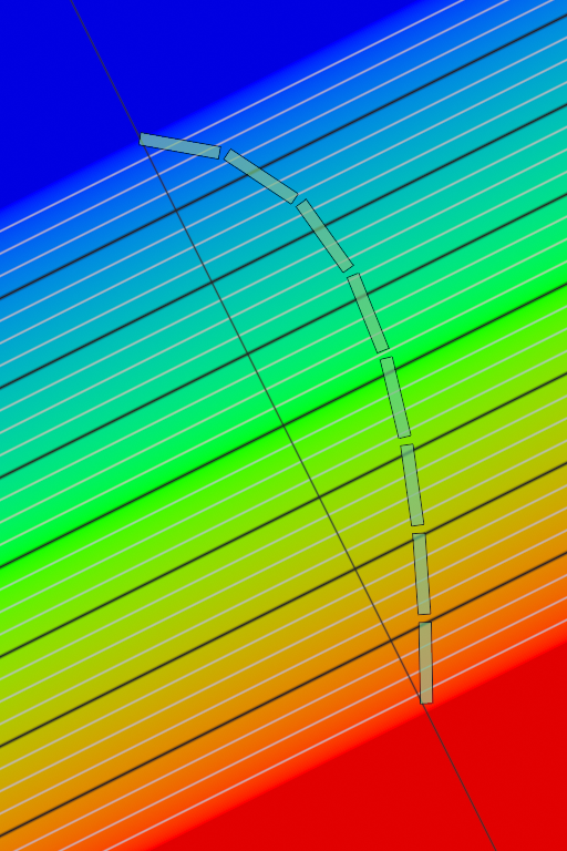
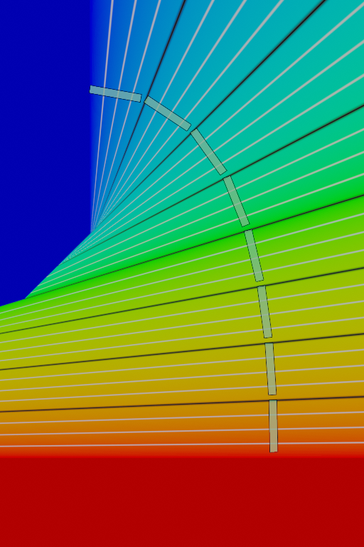
The simplest mapping method that existed since introduction of B-Bones is the Straight mapping. The vertex position is simply perpendicularly projected onto the line connecting the head and tail of the bone in the rest pose, clamped and divided by its length.
This is extremely fast to compute, which is important because the mapping is not cached, and works well if the bone is (almost) straight in the rest pose. However if the bone is significantly curved, as can be seen on the right, the mapping doesn't make much sense. It results in bad deformation in the area of high rest curvature:
-
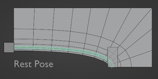
Bbone-mapping-rest.png -

Bbone-mapping-def-straight.png
Curved Mapping
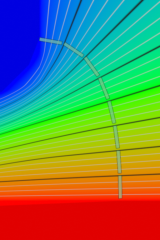
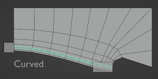
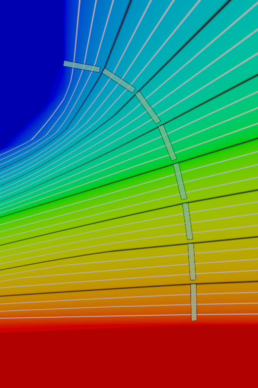
In order to fix the deformation issues it is necessary to take the rest pose curvature of the bone into account. This is implemented by the Curved mapping, which produces significantly better deformation in the same test case:
On the outside of the curve to the right this mapping corresponds to an orthogonal projection on the curve, while on the inside to the left the lines eventually align parallel to the center (green) line.
BSP Search
The core idea of this mapping is to do orthogonal projection on the curve itself, instead of the straight line that connects the end points. However, there is no analytical solution for projection on a Bézier curve, so it is necessary to use an approximation.
Therefore, the implementation uses the already constructed segment joint sequence to form a binary space partitioning tree that can be used to easily narrow down the mapping to a single segment through a binary search. Within the segment a simple linear interpolation between the BSP planes can be used to determine the final mapping point.
Smoothing
The BSP search alone produces a curved mapping, but it has a major issue: a discontinuity located along the evaluate surface, where the mapping abruptly jumps from the nearest end of the curve to a point in the middle. This discontinuity can result in vertex pops if shape keys are used to deform the affected area. Therefore it is necessary to smooth the discontinuity.
The employed smoothing scheme is completely heuristic and was developed by trial and error. The main idea is that all BSP planes that were checked during the search are processed in the reverse order from leaf to root, and push the mapped position in order to reduce the local gradient to the ideal slope, defined as the slope that occurs at the curve itself. Since smoothing never increases the slope, points on the outside of the curve where the gradient is lower than the ideal are not affected at all.
The smoothing calculation is based on comparing two values: the current distance of the mapped position from the plane in the head-tail space, and the ideal distance computed based on the distance of the point from the plane in 3d space and the ideal gradient slope.
The ratio of the distances is used to compute the slope coefficient that controls the onset of the smoothing as the gradient slope increases going from the outside to the inside of the curve. The ratio (minus 1) is asymptotically clamped from [0..infinity] into the [0..1] range, with a heuristic tuning coefficient (3.0) governing how fast the onset from 0 happens to avoid sharp bends or wobble in the transition from the no smoothing zone near the curve.
The 3d distance on its own is used to compute the distance coefficient, which falls off from 1 at the plane to 0 and controls how wide is the smoothed transition in the 3d space. This transition band radius is interpolated exponentially from exactly 1 segment at the BSP tree leaves to 0.222 of the distance between the curve end-points at the root BSP plane. The coefficient is also smoothed to ensure a continuous derivative at the transition to 0 to avoid sharp bends in the mapping isolines at the outside boundary of the smoothing band, with a transition sharpness tuning coefficient 7.0.
Finally, the slope and distance coefficients are multiplied together and used as a blend factor to push the current mapped position to the slope based ideal position.
Raw BSP
Bbone-mapping-curved-bsp.png Unsmoothed coefficients
Bbone-mapping-smooth-raw.png Slope 3.0
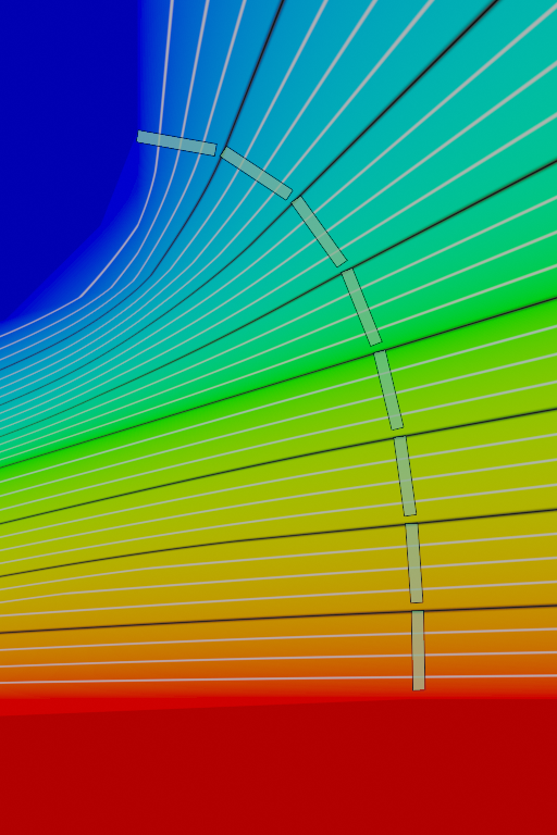
Bbone-mapping-curved-raw-ssm.png Distance 7.0 (Final)
Bbone-mapping-curved.png
This blend file contains a material node based model of the mapping and
was used to develop it, as well as render the above pictures:
